Code
knitr::opts_chunk$set(fig.align = 'center',
                      fig.show = 'hold', fig.width = 6.5, fig.height = 4,
                      out.width = "97%",
                      cache = FALSE)

library(ggplot2)
theme_set(theme_bw())With modern macro objectives and modern cameras some of the traditional rules-of-thumb for macro photography need to be reassessed. In this page, I summarize what I have learnt through experience and from various sources. The account is based on the micro-four-thirds lenses and adapted vintage lenses and the micro-four-thirds cameras that I use. This notes will continue envolving as I learn new things.
OM-1 digital, BSI sensor, sensor-shift high resolution
In this page code chunks can be “folded” so as to decrease the clutter. Above each plot, table or other R-code output you may find one or more “folded” code chunks signalled by a small triangle followed by “Code”. Clicking on the triangle “unfolds” folded chunks making the R code that produced the printed values, plots or tables visible. Clicking on the same icon on an “unfolded” chunk, folds it hiding the code.
The code when visible in the chunks can be copied by clicking on the top right corner, where an icon appears when the mouse cursor hovers over the code listing.
The </> Code drop down menu to the right of the page title makes it possible to unfold and fold all code chunks in the page and to view the Quarto source of the whole web page.
knitr::opts_chunk$set(fig.align = 'center',
fig.show = 'hold', fig.width = 6.5, fig.height = 4,
out.width = "97%",
cache = FALSE)
library(ggplot2)
theme_set(theme_bw())As discussed below, the depth of field in close-up and macro photography tends to be shallower than the depth of the object being photographed. I give here two examples, differing in magnification, none of them qualifying as true macro as the magnication is considerably less than 1:1. Anyway, a single photograph at f:5.6 leaves in both cases a large part of the subject out-of-focus.
We can take a series of photographs gradually shifting the focus (focus bracketing) and then combine the in-focus bits from each photograph in this “stack” into a single combined image with a much deeper region of the subject in focus. The stacking can be done off-camera with software (e.g., Helicon Focus) or in-camera in the case of the OM-System/Olympus mirrorless cameras.


Modern macro objectives and modern cameras are complex, and, thus, the traditional rules-of-thumb for macro photography need to be in part revised. Modern macro objectives rely on internal focusing mechanisms for close focusing instead of on the displacement of the optics as a whole away from the sensor or film. Given that for digital sensors, in contrast to film, an angle of incidence of light deviating from the normal can degrade image quality, most lenses designed for mirrorless cameras tend to be telecentric towards their rear end (telecentric means that the light beam does not expand, or expands less, than in the case of a simple lens as the distance increases. Some modern macro objectives are also telecentric at their front, to increase the working distance between the front of the objective and the subject relative to that of a simple lens of the same focal length. These developments alter how changes in magnification affect the effective f-value making the simple optical formulae even less useful than in the past. The result is that the nominal f-number of an objective, describing its aperture when focused at infinity, does not inform reliably about the lens aperture at macro magnifications.
Modern cameras like the OM-D OM-1 have features that affect their use for macro photography. Some, add new capabilities, such as image stabilization and fast auto-focus, that facilitate work and just expand possibilities by shifting the situations under which hand-holding the camera is feasible. The situation is less straightforward in relation to focus-bracketing (including focus-stacking), because the way it is controlled in-camera is different from focusing rails. In the case of focusing rails, manual and motorized, the change in focus-point is achieved by moving the whole camera to change the camera to subject distance, which is doable at short focusing distances. At high magnification, manual focusing rails or manually adjusting the focus at the objective are difficult to achieve without disturbing the position of the camera. Motorised rails are bulky and expensive. Modern Olympus/OM-System cameras have supported for several years automated focus bracketing using the autofocus mechanism of objectives. Optically, when focus stacking is the intended use of the focus-bracketed photographs, it is also preferable to adjust focus distance at the objective than by displacing the camera as it keeps the viewpoint unchanged. Camera based focus bracketing in the OM-1 camera is extremely fast, which is a huge benefit with live subjects in the field. However, when using a focusing rail displacement distances are given in constant units, such as millimetres, while in Olympus/OM-System cameras the focus step depends on the distance, f-number and lens focal-length. This helps by keeping the scale in use to 10 discrete steps 1 to 10, in the OM-1, but makes it more difficult for the user to guess what is a good setting for each individual situation.
A disadvantage of modern macro objectives is that the use of macro extension tubes to increase magnification can lead to a very significant degradation in optical performance. This explains why Olympus never offered macro extension tubes for the MFT mount. In contrast, as the FT D.Zuiko 50 mm f:2.0 macro objective did not have an internal focusing mechanism, it could be used with an extension tube, supplied by Olympus for the FT mount.
Below I summarize my own exploration of this subject, and what I have learnt both from various sources and through experimentation. This page is work in progress and I intend to revise and expand it in the future.
Modern “pro” objectives are corrected over a broader range of focusing distances than older designs, like those from the OM system of film cameras from the 1970’s to 1990’s, or cheaper modern designs, like some of the Venus Laowa or other modern even cheaper Chinese optics.
To achieve fast autofocus, the mass of the moving optics has to be lowered, thus modern autofocus objectives use internal focusing mechanisms, and sometimes also internal zoom mechanisms. Optical image stabilization adds the need for additional optical groups that move separately from those implementing focusing.
The resolution of digital camera sensors is much higher than that of film, and to be exploited requires higher image resolution from objectives. Modern Pro objectives from Olympus/OM-System are designed to resolve 100 MPix or more on a MFT sensor, which makes sense given that the sensor-shift high-resolution mode of OM-D cameras can already produce photographs at an 80 Mpix resolution.
An objective like the M.Zuiko 90mm f:3.5 able to produce very high quality images from infinity to a very high magnification was unheard of in the past. In the Olympus OM film system from the 1980’s, several different objectives were needed to cover this range of magnifications, with individual objectives optimized for different limited ranges of magnification.
Before the availability of highly effective anti reflection coatings, air-glass interfaces had to be few, as reflections at each interface significantly decreased image quality. Either elements had to be cemented into fewer groups or the number of elements kept low. An uncoated air-glass interface reflects about 4% of the light, making it impossible to build an objective like the M.Zuiko 90 mm f:3.5 with 26 such interfaces: \(0.96^{26} = 0.346\).
The pupil ratio is the ratio between the apparent diameter of the diaphragm opening measured at the back (exit pupil) and front (entrance pupil) of a lens. For lenses of simple construction the ratio is 1.0 and does not vary when the focus point is changed by moving the whole objective away or towards the film or sensor. The Zuiko 50mm f:3.5 Macro from the film OM System was the first Olympus objective with a group that moved with respect to other groups to implement corrections that make the lens perform well at a very broad range of focus distances. This is an objective where focusing is implemented by moving the whole optics, and the lens as a whole extends by 15mm, and the optics move even further, when changing the focus from \(\infty\) to 0.22m to achieve \(0.5\times\) magnification. Larger magnification can be achieved by inserting a macro extension tube between the objective and the camera.
In modern objectives containing multiple groups that move with respect to each other, not only pupil ratios frequently differ from 1.0, but in addition, the pupil ratio can change when the focus point is shifted. When the Four-Thirds mount was announced and Olympus advertised the first FT objectives, a feature that was highlighted was that these new objectives, designed specifically for digital cameras, were telecentric on the sensor side. This would be relevant for the exit pupil if the rear element of the objectives moved during focusing, which is not the case for the three M.Zuiko Macro objectives. Neither the front nor the back of these objectives moves, focusing is achieved entirely by movement of elements or groups internal to them. The pupil ratio is difficult to measure in telecentric lenses because of parallax likely affecting differently the measurements of entrance and exit pupils.
The usual calculation of effective aperture seems not to be applicable to modern and complex objectives like the M.Zuiko 90mm f:3.5 Macro based on the apparent pupil ratio measurements. This is not surprising as the M.Zuiko 90 mm is most likely of a telecentric design as most MFT and FT objectives are. This lens has an internal focusing mechanism, thus the position of the front and rear elements of the lens does not change. In principle, deviations could be accounted by incorporating the pupil ratio. This approach, breaks down in the case of telecentric objectives because of the impossiblity to correctly measure the pupil ratio by sight using a ruler. We can compare the specifications given in the manual, provided either as effective aperture values or as required exposure compensation, to the theoretical values computed.
| Magnification | f.nom | f.eff | f.theor | mode | pupil ratio |
|---|---|---|---|---|---|
| \(2.0\times\) | \(5.0\) | \(8.0\) | \(16.6\) | S-MACRO | \(\approx 0.86\) |
| \(1.0\times\) | \(5.0\) | \(6.3\) | \(15.4\) | S-MACRO | \(\approx 0.48\) |
| \(0.5\times\) | \(5.0\) | \(5.0\) | \(7.9\) | S-MACRO | \(\approx 0.85\) |
| \(2.0\times\) | \(3.5\) | \(-\) | \(-\) | other | \(\approx 0.86\) |
| \(1.0\times\) | \(3.5\) | \(4.5\) | \(7.9\) | other | \(\approx 0.86\) |
| \(0.5\times\) | \(3.5\) | \(4.0\) | \(5.7\) | other | \(\approx 0.86\) |
| \(0.25\times\) | \(3.5\) | \(3.5\) | \(4.6\) | other | \(\approx 0.72\) |
| focus at \(\infty\) | \(3.5\) | \(3.5\) | \(3.5\) | other | \(\approx 0.82\) |
Using manual focus and the non S-MACRO modes, on an uniformly illuminated surface (a computer monitor) the EV from the auto-exposure changes very little, agreeing with the effective f-values reported in the documentation. This is for a macro objective very useful behaviour, because if we do the computations backwards we see that at \(1\times\) magnification the M.Zuiko 90mm, behaves as an f:2.0 objective would. In S-MACRO mode exposure changes as magnification increases, and the exposure is almost the same at the same magnification and nominal f-number. So, also in this case the M.Zuiko 90mm f:3.5 is behaving as an objective with a larger maximum aperture.
Diffraction limits the maximum resolution achievable at small effective apertures, i.e., as the effective f-number increases, not according to the nominal f-number. From the perspective of macro photography that the maximum nominal aperture is f:3.5 is of little importance, as the effective aperture is large enough to allow accurate focusing and because in most cases a smaller aperture is needed to increase the depth of field by partly closing the diaphragm.
In the M.Zuiko 60 mm f:2.8 the decrease in effective aperture is less than expected but more than in the M.Zuiko 90 mm f:3.5, so that at \(1\times\) magnification, the effective aperture of the 90mm f:3.5 objective is larger than that of the 60mm f:2.8 lens. In the S-MACRO setting of the 90 mm lens, with a nominal aperture of f:5.0, the effective aperture is only slightly smaller than in the 60 mm f:2.8. Thus, at magnifications of \(0.25\times\) or more, the 90 mm f:3.5 objective has a larger effective aperture than the 60 mm f:2.8. The 60 mm f:2.8 is an excellent macro objective, but it lacks the optical image stabilization, the large working distance and the fast auto-focus of the M.Zuiko 90mm f:3.5.
| Magnification | f.nom | f.eff | f.theor | mode | pupil ratio |
|---|---|---|---|---|---|
| \(1.0\times\) | \(2.8\) | \(5.6\) | \(12.4\) | - | \(\approx 0.29\) |
| \(0.5\times\) | \(2.8\) | \(4.4\) | \(5.4\) | - | \(\approx 0.54\) |
| \(0.25\times\) | \(2.8\) | \(3.8\) | \(3.7\) | - | \(\approx 0.74\) |
| focus at \(\infty\) | \(2.8\) | \(2.8\) | \(2.8\) | - | \(\approx 0.75\) |
In my experience, all three objectives, the 30 mm f:3.5, the 60 mm f:2.8 and the 90 mm f:3.5 handle without problems the 80 MPix high resolution mode of the OM-1 camera at least at their optimal f settings. The 90 mm outperforms, at the magnification I tested, the other two objectives at smaller apertures. In the case of the 30 mm f:3.5 macro objective, the large pupil ratio seems to explain the rather similar effective aperture at \(1\times\) magnification compared to the other two objectives. This small objective is difficult to use at high magnification because of the small working distance. However, at moderate magnifications it performs well. All three objectives perform very well fully open with a flat focus plane.
| Magnification | f.nom | f.eff | f.theor | mode | pupil ratio |
|---|---|---|---|---|---|
| \(1.25\times\) | \(3.5\) | \(7.1\) | \(6.4\) | - | \(\approx 1.5\) |
| \(1.0\times\) | \(3.5\) | \(5.6\) | \(-\) | - | $$ |
| \(0.5\times\) | \(3.5\) | \(4.5\) | \(-\) | - | $$ |
| \(0.25\times\) | \(3.5\) | \(4.0\) | \(-\) | - | $$ |
| focus at \(\infty\) | \(3.5\) | \(3.5\) | \(3.5\) | - | \(\approx 2.9\) |
Modern objectives are complex. The M.Zuiko 90 mm f:3.5 macro, released in 2023, has 18 elements in 13 groups, and some groups move relative to others, during focusing, for the S-MACRO mode, and for optical image stabilization. The M.Zuiko 60 mm f:2.8 macro, released in 2012, has 13 elements in 10 groups, internal focusing and no optical stabilization. The M.Zuiko 30 mm f:3.5 macro, released in 2016, has seven elements in six groups. The Zuiko OM Zuiko 50mm f:3.5 Macro, released in 1973, has five elements in four groups. At moderate magnification it has surprisingly good resolution, a flat focus plane, and no distortion. If properly focused (I use the digital magnifier in camera) it performs very well also with the diaphragm fully open.
| Magnification | f.nom | f.eff | f.theor | mode | pupil ratio |
|---|---|---|---|---|---|
| \(1.0\times\) | \(3.5\) | \(7.1\) | \(-\) | - | \(-\) |
| \(0.5\times\) | \(3.5\) | \(5.6\) | \(5.3\) | - | \(\approx 1.0\) |
| \(0.25\times\) | \(3.5\) | \(4.5\) | \(4.4\) | - | \(\approx 1.0\) |
| focus at \(\infty\) | \(3.5\) | \(3.5\) | \(3.5\) | - | \(\approx 1.0\) |
In the M.Zuiko Macro objectives the pupil ratio seems to change with focusing distance. In the OM Zuiko 50mm f:3.5 Macro from the 1970’s, the the pupil ratio is constant and equal to 1. While the three M.Zuiko objectives have an internal focusing mechanism, the OM objective extends when focusing. This objective has a maximum magnification of \(0.5\times\) by itself but can be used together with macro extension tubes with good results. The use of macro extension tubes with the M.Zuiko lenses is problematic given their construction, and Olympus/OM-System does not offer extension tubes. The M.Zuiko 90 mm f:3.5 can be used with teleconverters to increase the magnification to \(4\times\), which given the small MFT sensor size, yields the same field of view as \(8\times\) magnification on a camera with a full-frame sensor.
In all M.Zuiko objectives, except the 30 mm f:3.5, the specified effective apertures are wider than the theoretical ones, but my estimates of the pupil ratio are very uncertain. With such complex lens designs it is difficult discover how the wider effective apertures are achieved given that measuring the pupil ratio becomes very difficult.
The M.Zuiko lenses do have microprocessors and built-in memory with firmware including stored information used in-camera for various corrections. Controls are implemented by wire and thus it would be possible that the aperture position or size changes concurrently with the internal focusing mechanism, but this seems unlikely.
I have been unable to find information on the depth of field for the M.Zuiko 90mm f:3.5 Macro objective, like that published by Olympus for the M.Zuiko 60mm f:2.8 Macro, M.Zuiko 30mm f:2.8 Macro, and the old Zuiko 50mm f:3.5 Macro. The tables take into account the image size, using 1/60mm for M.Zuiko and 1/30mm for Zuiko OM. With a pixel pitch of \(3.37\,\mathrm{\mu m}\) a minimum value to use would be \(10\,\mathrm{\mu m}\) while 1/60mm is \(16.6\,\mathrm{\mu m}\) and 1/30mm \(33.3\,\mathrm{\mu m}\). In the case of sensor-shift high resolution mode, it would sensible to base DOF on a smaller circle of confusion of \(\approx5\,\mathrm{\mu m}\). Table 9 Provides estimates of depth of field as a function of effective aperture. Using the values from the section above, including the decrease in f-number due to camera settings, and looking up the DOF from Table 9 based on the magnification in use should provide a reasonably good estimate. Of course, it is also possible to preview the depth of field through the camera, but the difference in resolution between the electronic view finder and actual image must be remembered. The higher the image resolution, the narrower is the apparent depth of field.
Experimentally measuring depth of field is beyond my capabilities and equipment.
Focus bracketing is controlled in the OM-1 camera by two settings: 1) focus differential expressed in what seems an arbitrary but monotonically increasing number in the range 1 (narrow) to 10 (wide), with default 5 and 2) depth of the stack as the number of frames in the range 1 to 15 or 999 (default 8 for stacking and 99 for bracketing).
Additionally, a delay or “charge time” between frames, to allow a flash to get ready in the range 0 to 30 s with 0.1, 0.2, 0.5, 1, 2, 4, 8, 15 and 30 s as possible values (default 0 s). With Olympus/OM-System flashes including the older FL-36R, the necessary delay is managed automatically and the setting can be left at zero. TTL-flash control is not supported in sensor shift high-resolution mode or focus bracketing, and with Olympus/OM-System flashes the switch to manual is automatic. When using third-party flashes like those in the Godox X-system, the flash control mode does not switch automatically to manual mode, and if left in the TTL setting, only the first photograph is well exposed, with subsequent flashes triggered at full power. My experience is with a Godox AD200 flash and a Godox Xpro O trigger.
For in-camera focus stacking, in the OM-1, the maximum number of frames is 15, and frames are captured both in front and behind the starting focus point. For focus bracketing, the maximum number of frames is 999 and all frames are taken moving the focus point away from the camera, starting from the initial position. The initial position is restored at the end of the bracketed series.
The focus differential setting in 1 to 10 is not expressed in a fixed scale. The actual shift of the focus point for one unit of focus differential is a function of the focusing distance, current diaphragm setting (nominal f-value) and possibly objective type or focal length. This makes estimating the depth in mm or m covered by a bracketed set of images difficult. On the other hand, it seems to keep the focus depth setting nearly proportional to the observed depth of field available with the settings currently in use. This is in fact excellent as it makes the suitable setting rather independent of the camera settings. The 1 to 10 scale for a given camera setting seems to be nearly linear in distance. In long stacks the step length seems to slightly increase as the focus point moves away from the camera.
I have not found detailed information in the camera manual or on-line except for the Focus Bracketing Reference Sheet for the OM-1 with the M.Zuiko 60mm f:2.8 Macro lens from Chris McGuinnis.
Because of this, I have done some measurements for the OM System M.Zuiko 90mm f:3.5 Macro PRO on the Olympus OM-1 Digital Camera. Because of diffraction, f-values between 3.5 and 8 yield higher resolution than smaller apertures. In the high-resolution mode of the camera, diffraction will be more limiting than at the base resolution.
The first tests confirmed that at a given camera setting, the displacement increases linearly from 1 to 10. Thus, it is enough to measure the step size and only one focus differential setting, for each camera setting of interest.
| Magnification | f | f.eff | DOF (mm) | FD = 1 (mm) | frames (mm\(^{-1}\)) |
|---|---|---|---|---|---|
| \(2\times\) | \(5.0\) | \(8.0\) | \(\approx 0.126\) | \(\approx 0.015\) | \(\approx 67\) |
| \(8.0\) | \(13\) | \(\approx 0.2\) | \(\approx 0.03\) | \(\approx 33\) | |
| \(22.0\) | \(35\) | \(\approx 0.52\) | \(\approx 0.070\) | \(\approx 14\) | |
| \(1\times\) | \(3.5\) | \(4.5\) | \(\approx 0.19\) | \(\approx 0.035\) | \(\approx 29\) |
| \(8.0\) | \(10\) | \(\approx 0.42\) | \(\approx 0.075\) | \(\approx 13\) | |
| \(22.0\) | \(28\) | \(\approx 1.1\) | \(\approx 0.200\) | \(\approx 5\) | |
| \(0.5\times\) | \(3.5\) | \(4.0\) | \(\approx 0.5\) | \(\approx 0.275\) | \(\approx 4\) |
| \(8.0\) | \(9.1\) | \(\approx 1.1\) | \(\approx 0.330\) | \(\approx 3\) | |
| \(22.0\) | \(25\) | \(\approx 3.3\) | NA | NA |
Table 5 shows computed values for DOF. These roughly match what I see in the photographs of a high resolution scale, with marks every \(0.1\,\mathrm{mm}\), on a plane slanted at 30 degrees. In most cases, at magnifications of more than \(0.5\times\), FD = 2, seems to ensure a reasonable overlap of the sharp regions in successive frames, while FD = 5 leaves a slightly out-of-focus band between successive frames. Thus, it seems that FD = 3 matches approximately the actual DOF. FD = 1 or FD = 2 should be good for focus stacking. At the highest magnifications it may be possible to to use FD = 3 or FD = 4 with a very stable copy stand in a vibration free setting.
With modern lenses, it is better to rely on manufacturers’ specification- and instruction-sheets to obtain the effective f-values than to rely on tables or simple formulas that ignore the pupil ratio. As measuring the pupil ratio of some modern telecentric objectives is difficult, the use of formulas that take it into account the pupil ration, may also fail to provide a reliable estimates of the effective f-number at different magnifications.
Depth of field at high magnification can be predicted using formulae, but it is necessary to keep in mind that one has to use the effective f-number for the computations of table look-up.
Deciding on the focus differential to use and number of frames should be simpler than how it looks like, but lack of detailed information hinders it. It seems that the only way out is to follow McGuinnis example and rely on experimentation to work out some guidelines. The preliminary measurements that I have done, are not enough.
When this new macro objective was announced, on-line reviews were quickly published. A widespread criticism was that f:3.5 was too slow an aperture for a macro objective. As discussed above this could have been true for a lens of simpler design. What matters is the true effective aperture and the M.Zuiko 90 mm delivers a large enough one.
Lens design is full of compromises. Achieving the exceptionally effective image stabilization and fast auto-focus make it necessary to keep the mass of the moving optical groups as low as possible. In macro photography depth of field is very shallow and very large apertures are normally of little use. This lens has what looks like an unusual/original design that allows it to perform better than any other macro lens when used handheld. It is also a telephoto lens, with a full-frame-equivalent focal length of 180 mm, for which f:3.5 is not particularly slow. This lens is unique in that it can reach a very high magnification of 2x, on the small MFT sensor. At this high magnification the hit rate when used handheld is rather low, in part because of subject movement. It can be also used with the 1.4x and 2.0x teleconverters, to achieve up to x4 magnification. In this case a tripod or other firm support is needed, and diffraction may start limiting resolution. This is most noticeable when using the 80 MPix mode at very high magnification. It is still an incredible technological feat that the same objective performs well from infinity focus all the way to x4 magnification.
Is the M.Zuiko 90 mm f:3.5 Macro too expensive? We do not know how much it costs to manufacture it, we only know that it is unique in its features. If one does not need the ability to take photographs handheld at high magnification, optically the cheaper M.Zuiko 60 mm f:2.8 Macro is nearly as good a macro lens, with a shorter working distance that is anyway enough in most situations. One can use the sensor-shift high resolution modes without problems with either of these two lenses. The much cheaper 30 mm f:3.5 although achieving slightly higher magnification than the 60 mm f:2.8 is limited by the very short working distance that makes lighting difficult at high magnifications. At least my own copy of the M.Zuiko 30mm f:2.8 Macro, does seem to have slightly lower resolution than the other two macro lenses when used in the 80 MPix sensor-shift mode. The 90 mm f:3.5 Macro is weather sealed and can be used in the rain. The 60 mm f:2.8 is splash proof but the 30 mm f:3.5 is not.
If one is willing to use a fully manual lens and dispense with weather sealing, cheaper alternatives exist that reach a high magnification of 2x and even 5x with different performance compromises, e.g., from Venus Laowa. Personally, I find adjusting the aperture or focus directly on a lens problematic when working at very high resolution as the slightest shift in the position of the lens or subject is enough to ruin a photograph. Even when using manual focus, the ability to adjust focus and all other settings remotely without touching the camera or the lens is extremely useful. It is of course possible to use a manual lens for close-up photography of insects, as I have done with a film camera years back using a flash. However, adapted lenses and even most of the in-production manual macro lenses lack an automatic diaphragm, and this lack is a big hindrance for manual focusing.
The sensor of the OM-1 has according to specifications 22.6 Mpix of which 20.4 Mpix are in effective use. The effective size of the captured iamge can be slightly less. The applied distortion corrections and slight cropping depend on the objective used. The OM-1 camera supports high-resolution modes based on sensor shift. These high resolution photographs are composed from eight images acquire in rapid succession displacing the sensor so that not only information is acquired for each pixel for the four RGBG channels, but also displaced by half a pixel. The result is an image with improved colour accuracy, less noise and higher resolution. As the size of the sensing area per pixel remains the same, it cannot be expected that the true resolution quadruples (double in each of x and y axes).
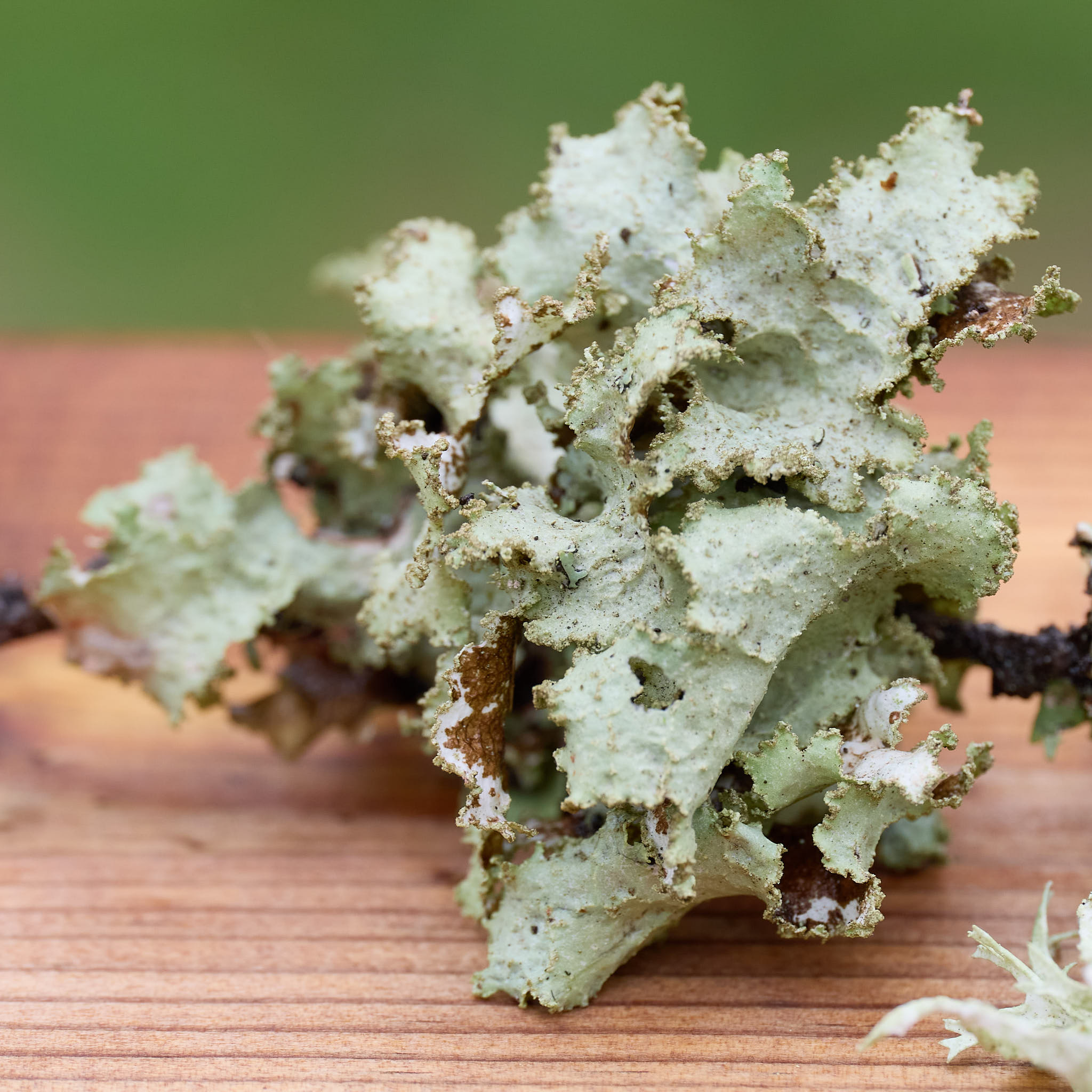
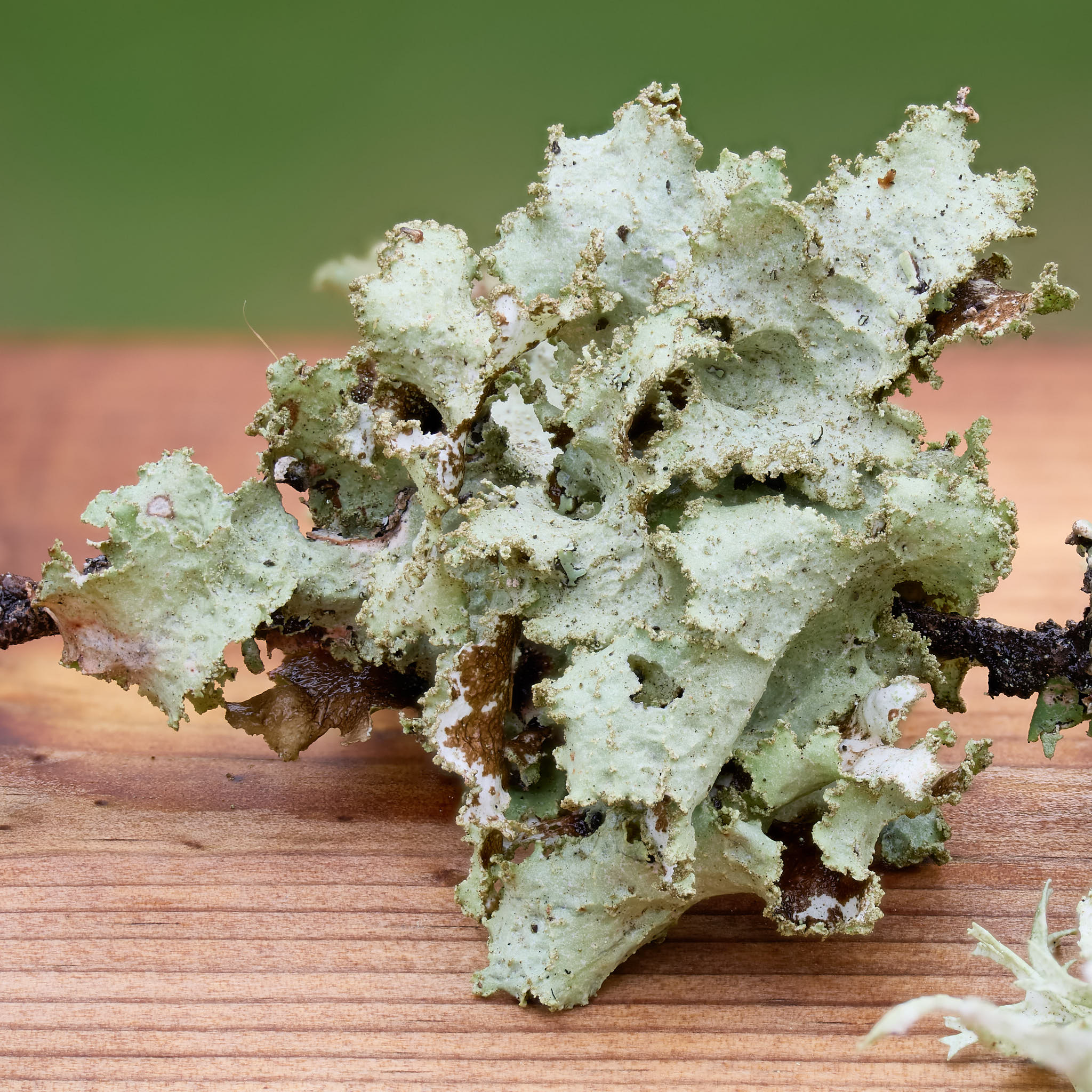
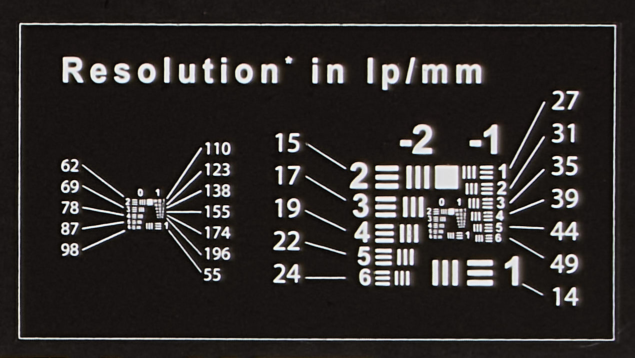
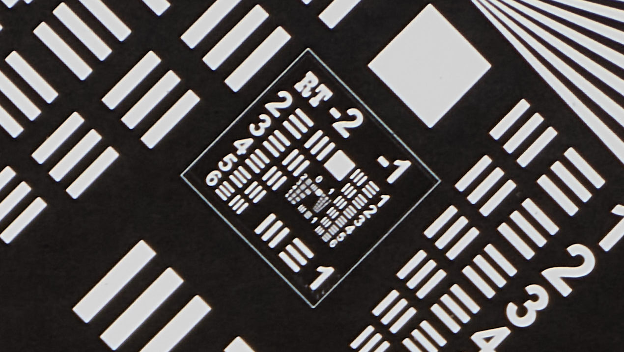
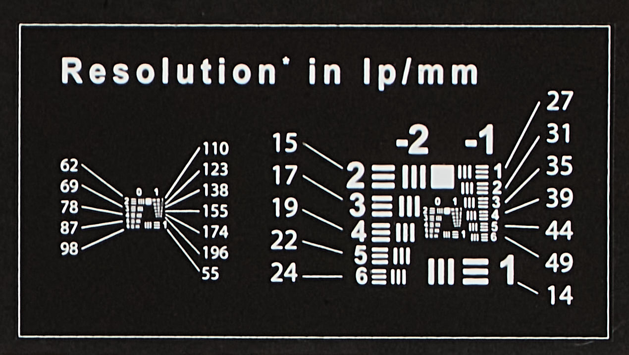
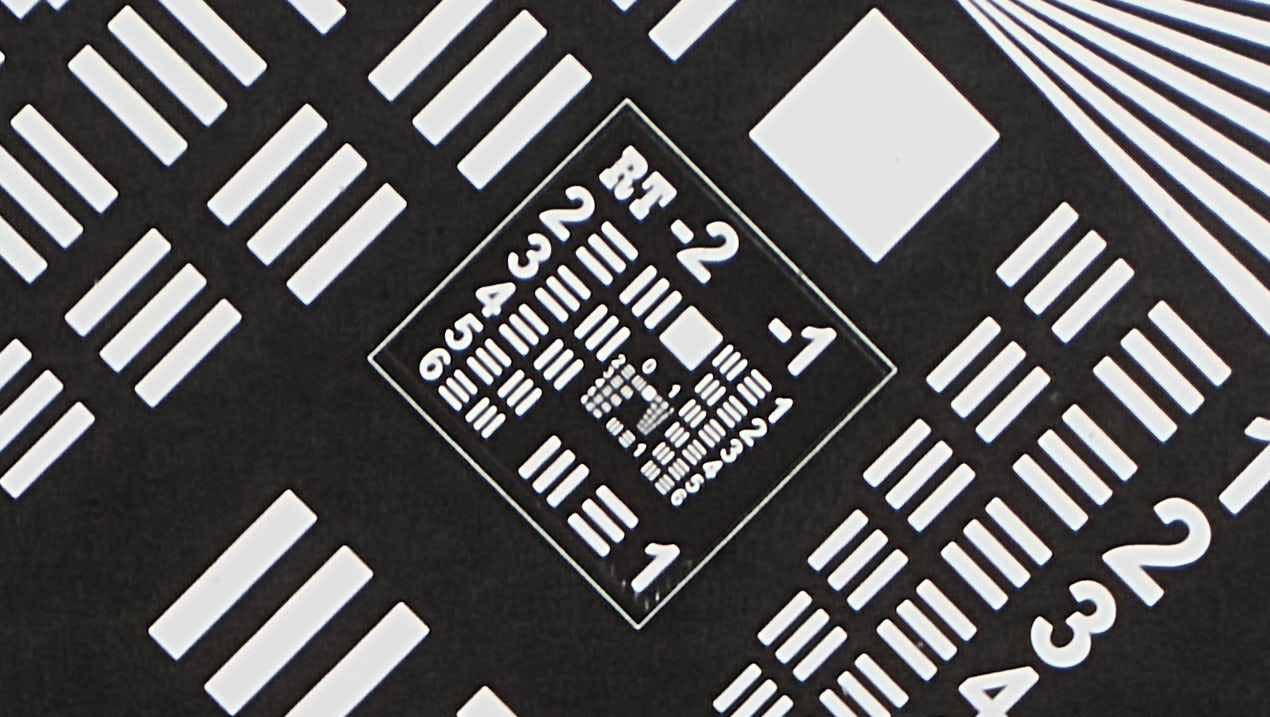
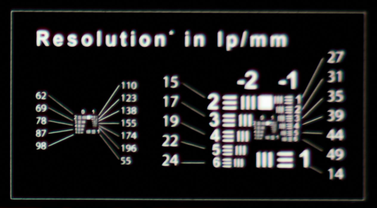
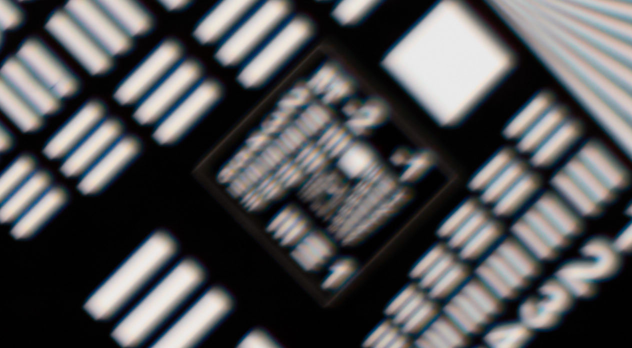
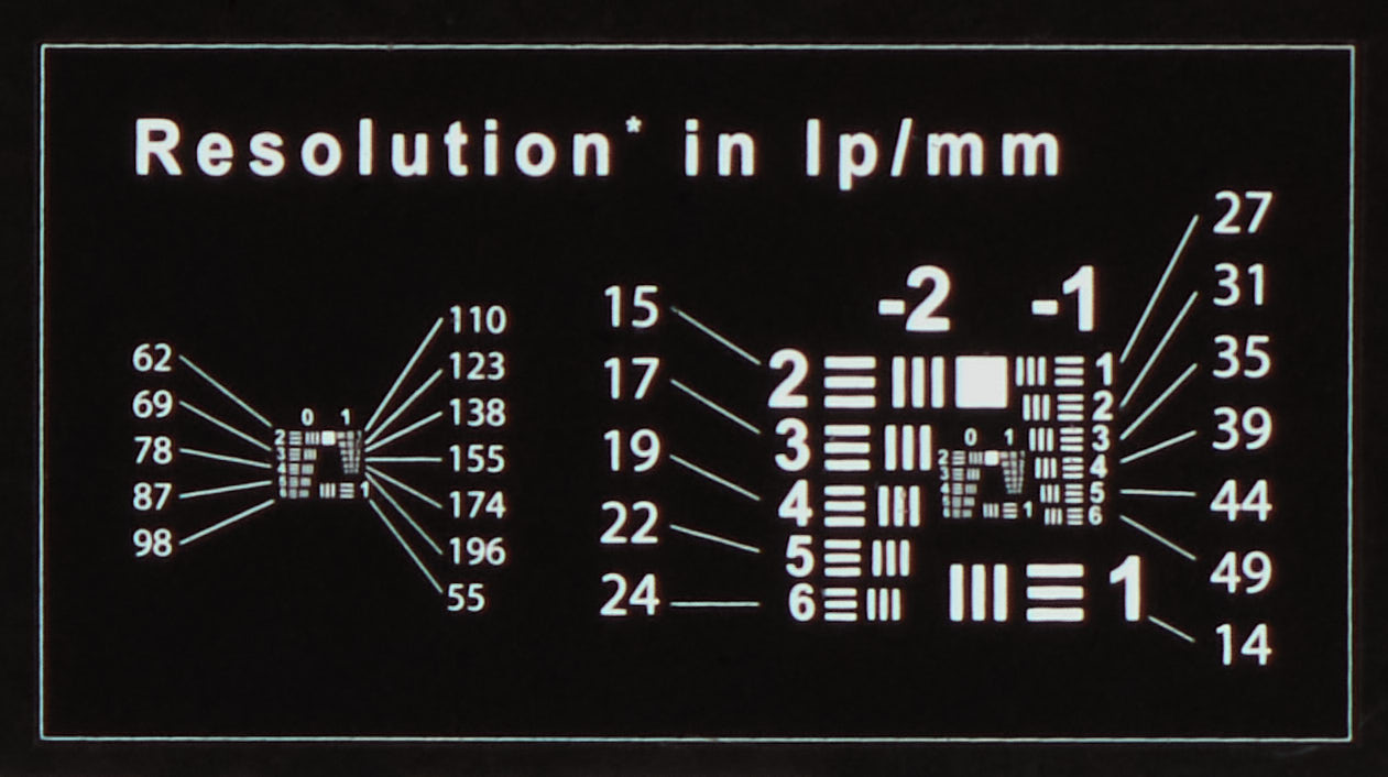
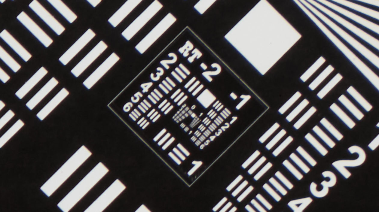
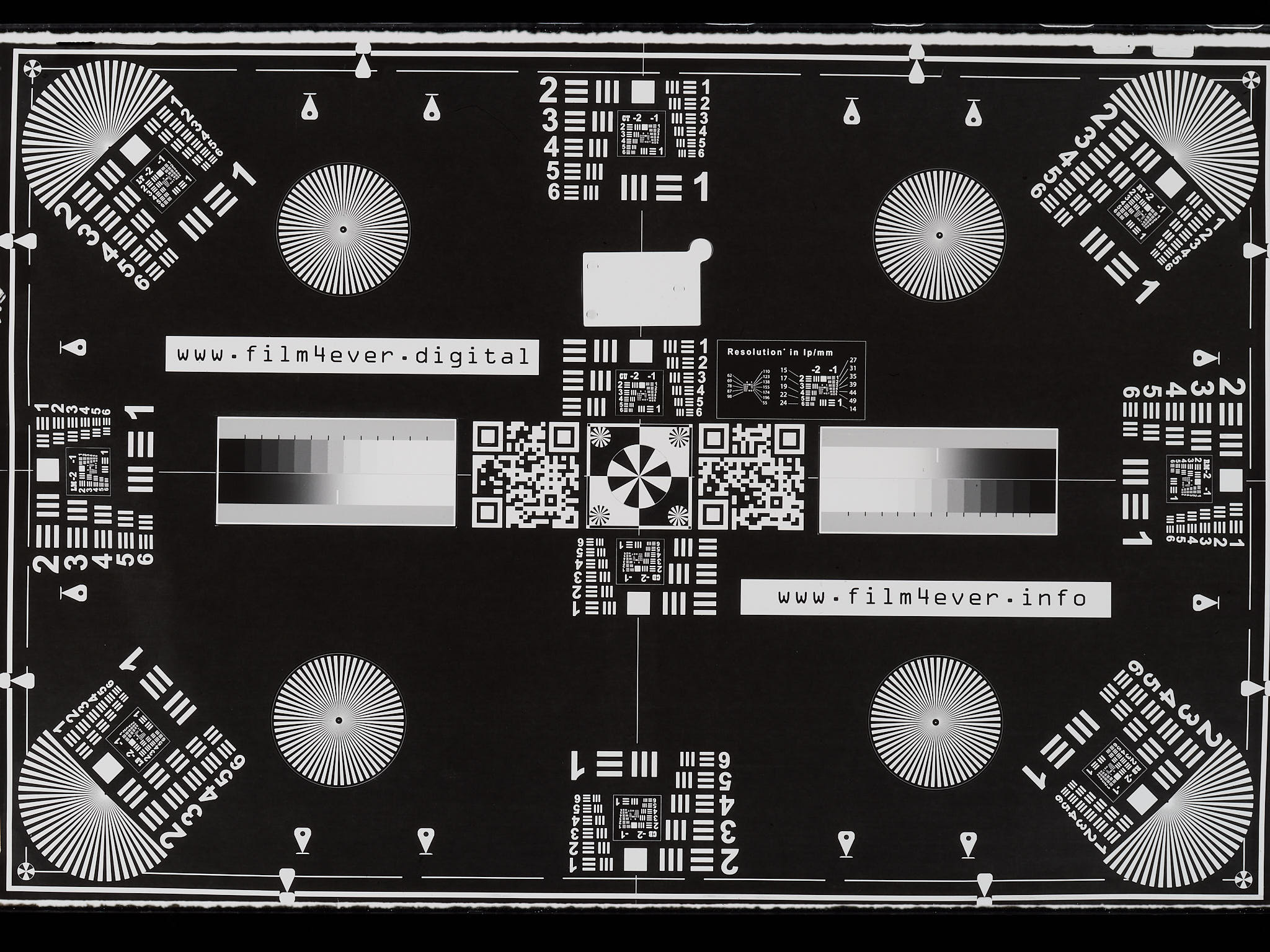
Using Vlads test target 35 mm on a Valoi 135 film holder transilluminated with an Elgato Key Light Mini I estimated the resolution achievable using the 80 Mpix sensor shift mode of the OM-1 camera. The target uses the USAF-1951 pattern as is based on a Adox 20 film. The values are for a magnification of approximately 1:2 given the difference in size of the sensor and target. The target has high contrast and the resolution reported is based on the size of the target pattern, not that of the sensor. The values shown should be interpreted as relative rather than as absolute values in lp/mm. The “80 Mpix mode” files have 10368 x 7776 pixels or 80.6 Mpx for a sensor size of 18 mm × 13.5 mm (22.5 mm diagonal), with an imaging area of 17.3 mm × 13.0 mm, giving a diagonal of 21.64 mm. The pitch of the square pixels on the sensor is 1.67 um or 600 pixels per millimetre. Figure 1 and Figure 2 show the outcome of the test. When the modulation transfer function (MTF) of a lens has a low value because of lost contrast and the target has very high contrast, it is possible to improve the apparent resolution of the image in post-processing. This can be seen in Figure 3 where the cropped photographs were both manually edited and also adjusted automatically when exported from raw to JPEG, which when examined appear to have higher resolution than that reported in Figure 1 and Figure 2.
usaf_lpmm.tb <-
  read.csv("objectives-copy-135-resolution.csv", comment.char = "#")

obj_type.map <- c(MZ90 = "MFT macro", MZ60 = "MFT macro", MZ30 = "MFT macro",
                  SG30 = "MFT with tube", SG60 = "MFT with tube",
                  Z50 = "adapted FF macro", NK24 = "adapted FF with tube")
usaf_lpmm.tb$obj.type <- obj_type.map[usaf_lpmm.tb$obj]ggplot(usaf_lpmm.tb, aes(f, centre80mpx, linetype = obj, colour = obj.type)) +
geom_hline(yintercept = 50, linetype = "dotted") +
geom_line() +
scale_x_log10(name = "Aperture (f-number)", breaks = c(2.8, 3.5, 4.5, 5.6, 8, 11, 16, 22)) +
scale_y_continuous(name = "Resolution on target (lp / mm)", limits = c(0, 80),
sec.axis = sec_axis(transform = ~ . * 2, name = "Resolution on sensor (lp / mm)")) +
labs(linetype = "Objective", colour = "Objective type")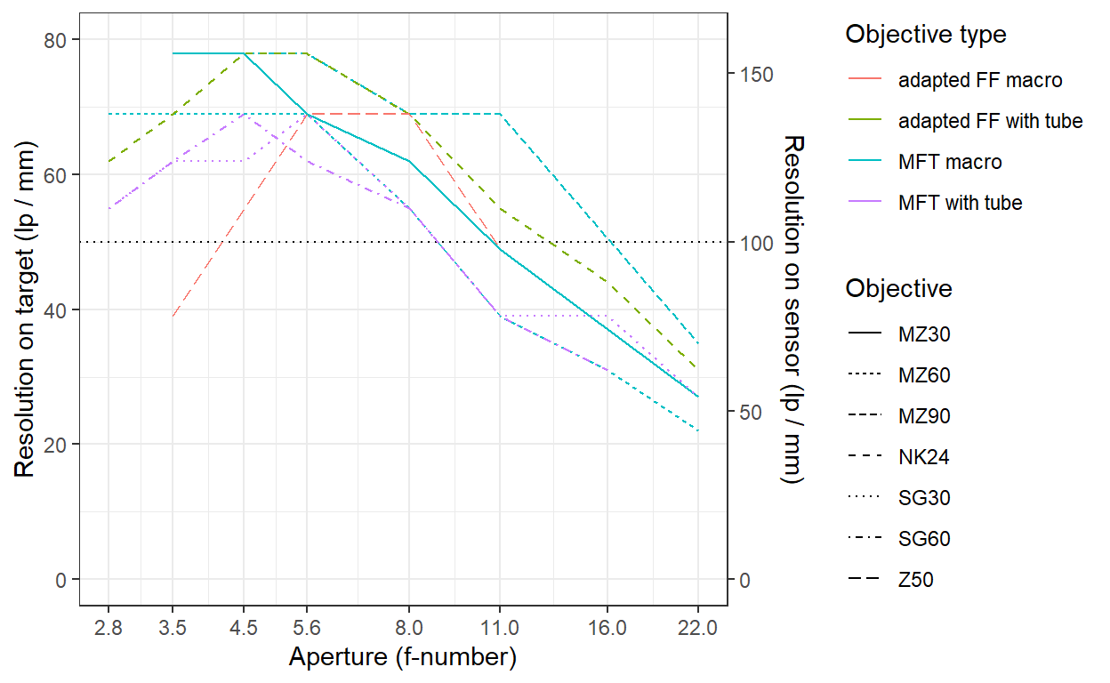
ggplot(usaf_lpmm.tb, aes(f, edge80mpx, linetype = obj, colour = obj.type)) +
  geom_hline(yintercept = 50, linetype = "dotted") +
  geom_line() +
  scale_x_log10(name = "Aperture (f-number)", breaks = c(2.8, 3.5, 4.5, 5.6, 8, 11, 16, 22)) +
  scale_y_continuous(name = "Resolution on target (lp / mm)", limits = c(0, 80),
                     sec.axis = sec_axis(transform = ~ . * 2, name = "Resolution on sensor (lp / mm)")) +
  labs(linetype = "Objective", colour = "Objective type")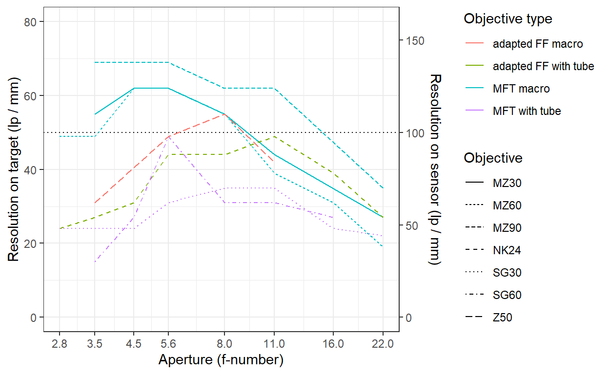
The biggest difference between M.Zuiko objectives and other objectives seem to be that Olympus/OM-System MFT Macro objectives tend to have very high resolution at this maximum aperture even far from the centre of the image. The Sigma MFT objectives when used with extension tubes perform very poorly at the corners of the frame, and performance improves when partly closing the diaphragm, but remains poor in the corners. Of the two full-frame objectives, the Nikkor performs very well at the centre of the frame and rather poorly at the corners. The Nikkor, like the Sigma lenses is not designed for Macro photography although it is corrected for close focusing (0.3 m). The Zuiko 50mm f:3.5 macro performs more evenly across the frame than the Nikkor, by having lower resolution at the center and and higher at the edges than the Nikkor. Out of all the objectives, the M.Zuiko 90mm f:3.5 clearly outperforms all other objectives tested and as mentioned above retains a very high resolution across a broader range of diaphragm apertures than the other objectives.
In the native resolution mode of the camera, or single frame photographs images files have 20.2 Mpix or 5184 x 3888 pixels for a sensor size of 18 mm × 13.5 mm (22.5 mm diagonal). A sensor imaging area of 17.3 mm × 13.0 mm, giving a diagonal of 21.64 mm. The pitch of the square pixels on the sensor is 3.34 um or 300 pixels per mm. The test described above was done at 80 Mpix resolution. However, with the camera used at its native resolution of 20.2 Mpix, differences among objectives are less obvious. The resolution capped near 100 lp / mm, but when lower closely matched that in Figure 1 and Figure 2. The horizontal black dotted line in these figures indicates the maximum resolution achieved by the camera sensor natively. A resolution of 100 lp / mm corresponds to 3 pixels per line pair. In contrast, the maximum resolution was at 80 Mpix 156 lp / mm, or 3.8 pixels per line pair. As mentioned above, doubling the resolution by simply displacing the position of the sensor pixels by half their pitch is not possible, as there is pixel overlap and information recovery involved. We see instead an increase of about 60% which together with reduced noise and better colour rendering improves image quality very significantly. The high resolution mode also reveals the limitations of lenses as well as a negative effect of diffraction at larger apertures.
The target I used is a very high contrast one, and especially at the corners with some of the worse performing lenses the contrast was very low, with the pattern of the target looking smeared and in some cases with colour halos. This was very different than the effect of diffraction at small apertures, which led to an even lowering of contrast and softening of the transition at the edge of the patterns. It is also relevant to remember that when the resolution is limited by the pixel pitch, the exact position of the pattern lines relative to pixels affects the apparent resolution. For each image I observed the four corner patterns and at least two of the patterns near the center of the target but in many cases deciding between two neighbouring resolution values was difficult.
In Figure 3 I reproduce small crops at full resolutiion of some of the photographs I used to estimate resolution of lenses. These are examples chosen based on the orientation of the text. For constructing the table patterns at each corner and three patterns near the center were evaluated from each photograph. Some corners were clearly sharper than others. While the photographs were only slightly edited before assessment, the crops in the figure were edited so as to improve as much as possible the apparent resolution. The intention of the figure is to show that a modern “Pro” level macro objective can achieve top performance both at the centre and far corners with the diaphragm fully open. The SIgma 30 mm 1:2.8 DN is a modern low price lens, no longer available new, designed for general photography that performs very well within its native focusing range. With macro extension tubes its performance deteriorates very significantly with the diaphragm fully open. After closing the diaphragm to f:5.6 it becomes usable at 1:2 magnification. The test done by photographing a flat target in the 80 Mpix mode is challenging for any lens as it is unforgiving about curvature of the focus plane. With other subjects and the setting at the native 20 Mpix mode of the camera all the tested lenses perform well in the centre of the image at least at some appertures.
The table below gives approximate effective f-numbers assuming ideal lenses with a pupil ratios of 1.5, 0.86 and 0.50 As shown above, the real pupil ratio of modern lenses is not constant. If is also clear above, that the actual effective apertures given by manufacturers for complex objectives differs from that based on the simple equations used to describe ideal simple lenses.
f_effective <- function(f.nominal, magnif, pupil.ratio = 1) {
  f.nominal * (magnif / pupil.ratio + 1)
}

depth_of_focus <- function(f.effective,
                           magnif,
                           focal.length,
                           pixel.pitch,
                           circle.of.confusion = pixel.pitch * 3){
  (2 * focal.length * (magnif + 1) / magnif) /
    ((focal.length * magnif) / (f.effective * circle.of.confusion) -
       (f.effective * circle.of.confusion) / (focal.length * magnif))
}

Airy_circle <- function(f.nominal, w.length = 550) {
  1.22 * w.length * f.nominal * 1e-3
}apertures <- c(1.4, 2.0, 2.8, 3.5, 4.0, 5.6, 8, 11, 16, 22)
names(apertures) <- paste("f", apertures, sep = ":")
magnifications <- c(2, 1, 0.5, 0.25, 0.1, 0.05)
names(magnifications) <- paste(magnifications, "x", sep = "")
sapply(apertures,
f_effective, magnif = magnifications, pupil.ratio = 1.5) |>
t() |> signif(3) |> knitr::kable()| 2x | 1x | 0.5x | 0.25x | 0.1x | 0.05x | |
|---|---|---|---|---|---|---|
| f:1.4 | 3.27 | 2.33 | 1.87 | 1.63 | 1.49 | 1.45 |
| f:2 | 4.67 | 3.33 | 2.67 | 2.33 | 2.13 | 2.07 |
| f:2.8 | 6.53 | 4.67 | 3.73 | 3.27 | 2.99 | 2.89 |
| f:3.5 | 8.17 | 5.83 | 4.67 | 4.08 | 3.73 | 3.62 |
| f:4 | 9.33 | 6.67 | 5.33 | 4.67 | 4.27 | 4.13 |
| f:5.6 | 13.10 | 9.33 | 7.47 | 6.53 | 5.97 | 5.79 |
| f:8 | 18.70 | 13.30 | 10.70 | 9.33 | 8.53 | 8.27 |
| f:11 | 25.70 | 18.30 | 14.70 | 12.80 | 11.70 | 11.40 |
| f:16 | 37.30 | 26.70 | 21.30 | 18.70 | 17.10 | 16.50 |
| f:22 | 51.30 | 36.70 | 29.30 | 25.70 | 23.50 | 22.70 |
apertures <- c(1.4, 2.0, 2.8, 3.5, 4.0, 5.6, 8, 11, 16, 22)
names(apertures) <- paste("f", apertures, sep = ":")
magnifications <- c(2, 1, 0.5, 0.25, 0.1, 0.05)
names(magnifications) <- paste(magnifications, "x", sep = "")
sapply(apertures,
       f_effective, magnif = magnifications, pupil.ratio = 0.86) |>
t() |> signif(3) |> knitr::kable()| 2x | 1x | 0.5x | 0.25x | 0.1x | 0.05x | |
|---|---|---|---|---|---|---|
| f:1.4 | 4.66 | 3.03 | 2.21 | 1.81 | 1.56 | 1.48 |
| f:2 | 6.65 | 4.33 | 3.16 | 2.58 | 2.23 | 2.12 |
| f:2.8 | 9.31 | 6.06 | 4.43 | 3.61 | 3.13 | 2.96 |
| f:3.5 | 11.60 | 7.57 | 5.53 | 4.52 | 3.91 | 3.70 |
| f:4 | 13.30 | 8.65 | 6.33 | 5.16 | 4.47 | 4.23 |
| f:5.6 | 18.60 | 12.10 | 8.86 | 7.23 | 6.25 | 5.93 |
| f:8 | 26.60 | 17.30 | 12.70 | 10.30 | 8.93 | 8.47 |
| f:11 | 36.60 | 23.80 | 17.40 | 14.20 | 12.30 | 11.60 |
| f:16 | 53.20 | 34.60 | 25.30 | 20.70 | 17.90 | 16.90 |
| f:22 | 73.20 | 47.60 | 34.80 | 28.40 | 24.60 | 23.30 |
apertures <- c(1.4, 2.0, 2.8, 3.5, 4.0, 5.6, 8, 11, 16, 22)
names(apertures) <- paste("f", apertures, sep = ":")
magnifications <- c(2, 1, 0.5, 0.25, 0.1, 0.05)
names(magnifications) <- paste(magnifications, "x", sep = "")
sapply(apertures,
       f_effective, magnif = magnifications, pupil.ratio = 0.5) |>
t() |> signif(3) |> knitr::kable()| 2x | 1x | 0.5x | 0.25x | 0.1x | 0.05x | |
|---|---|---|---|---|---|---|
| f:1.4 | 7.0 | 4.2 | 2.8 | 2.10 | 1.68 | 1.54 |
| f:2 | 10.0 | 6.0 | 4.0 | 3.00 | 2.40 | 2.20 |
| f:2.8 | 14.0 | 8.4 | 5.6 | 4.20 | 3.36 | 3.08 |
| f:3.5 | 17.5 | 10.5 | 7.0 | 5.25 | 4.20 | 3.85 |
| f:4 | 20.0 | 12.0 | 8.0 | 6.00 | 4.80 | 4.40 |
| f:5.6 | 28.0 | 16.8 | 11.2 | 8.40 | 6.72 | 6.16 |
| f:8 | 40.0 | 24.0 | 16.0 | 12.00 | 9.60 | 8.80 |
| f:11 | 55.0 | 33.0 | 22.0 | 16.50 | 13.20 | 12.10 |
| f:16 | 80.0 | 48.0 | 32.0 | 24.00 | 19.20 | 17.60 |
| f:22 | 110.0 | 66.0 | 44.0 | 33.00 | 26.40 | 24.20 |
In the normal mode, information is reconstructed from each group of four pixels, and consequently the effective pixel resolution is less, by approximately a factor of three (Table 9).
apertures <- c(3.5, 5.6, 8, 11, 16, 22, 32, 64, 128)
names(apertures) <- paste("f", apertures, sep = ":")
magnifications <- c(2, 1, 0.5, 0.25, 0.1, 0.05)
names(magnifications) <- paste(magnifications, "x", sep = "")
sapply(apertures,
       depth_of_focus, magnif = magnifications, focal.length = 90, pixel.pitch = 0.0035) |>
t() |> signif(3) |> knitr::kable()| 2x | 1x | 0.5x | 0.25x | 0.1x | 0.05x | |
|---|---|---|---|---|---|---|
| f:3.5 | 0.0551 | 0.147 | 0.441 | 1.47 | 8.09 | 30.9 |
| f:5.6 | 0.0882 | 0.235 | 0.706 | 2.35 | 12.90 | 49.4 |
| f:8 | 0.1260 | 0.336 | 1.010 | 3.36 | 18.50 | 70.6 |
| f:11 | 0.1730 | 0.462 | 1.390 | 4.62 | 25.40 | 97.1 |
| f:16 | 0.2520 | 0.672 | 2.020 | 6.72 | 37.00 | 141.0 |
| f:22 | 0.3470 | 0.924 | 2.770 | 9.24 | 50.90 | 195.0 |
| f:32 | 0.5040 | 1.340 | 4.030 | 13.40 | 74.00 | 284.0 |
| f:64 | 1.0100 | 2.690 | 8.070 | 26.90 | 149.00 | 577.0 |
| f:128 | 2.0200 | 5.380 | 16.100 | 54.00 | 302.00 | 1240.0 |
As in the sensor-shift high-resolution mode information is acquired for all colours at each pixel position, we set the circle of confussion the the pixel pitch (Table 10).
apertures <- c(3.5, 5.6, 8, 11, 16, 22, 32, 64, 128)
names(apertures) <- paste("f", apertures, sep = ":")
magnifications <- c(2, 1, 0.5, 0.25, 0.1, 0.05)
names(magnifications) <- paste(magnifications, "x", sep = "")
sapply(apertures,
       depth_of_focus, magnif = magnifications, focal.length = 90, circle.of.confusion = 0.0035) |>
t() |> signif(3) |> knitr::kable()| 2x | 1x | 0.5x | 0.25x | 0.1x | 0.05x | |
|---|---|---|---|---|---|---|
| f:3.5 | 0.0184 | 0.0490 | 0.147 | 0.490 | 2.70 | 10.3 |
| f:5.6 | 0.0294 | 0.0784 | 0.235 | 0.784 | 4.31 | 16.5 |
| f:8 | 0.0420 | 0.1120 | 0.336 | 1.120 | 6.16 | 23.5 |
| f:11 | 0.0578 | 0.1540 | 0.462 | 1.540 | 8.47 | 32.3 |
| f:16 | 0.0840 | 0.2240 | 0.672 | 2.240 | 12.30 | 47.0 |
| f:22 | 0.1160 | 0.3080 | 0.924 | 3.080 | 16.90 | 64.7 |
| f:32 | 0.1680 | 0.4480 | 1.340 | 4.480 | 24.60 | 94.1 |
| f:64 | 0.3360 | 0.8960 | 2.690 | 8.960 | 49.30 | 189.0 |
| f:128 | 0.6720 | 1.7900 | 5.380 | 17.900 | 98.80 | 380.0 |
https://olypedia.de/index.php?title=Zuiko_Auto-Macro_1:3,5/50_mm